Log Viewer

Time-series viewer for inspecting logged data channels

The Log Viewer lets you plot any combination of logged channels over time. It is useful for verifying data quality before tuning, diagnosing engine behaviour, and checking that your logs contain the conditions you need for a given tuning page.

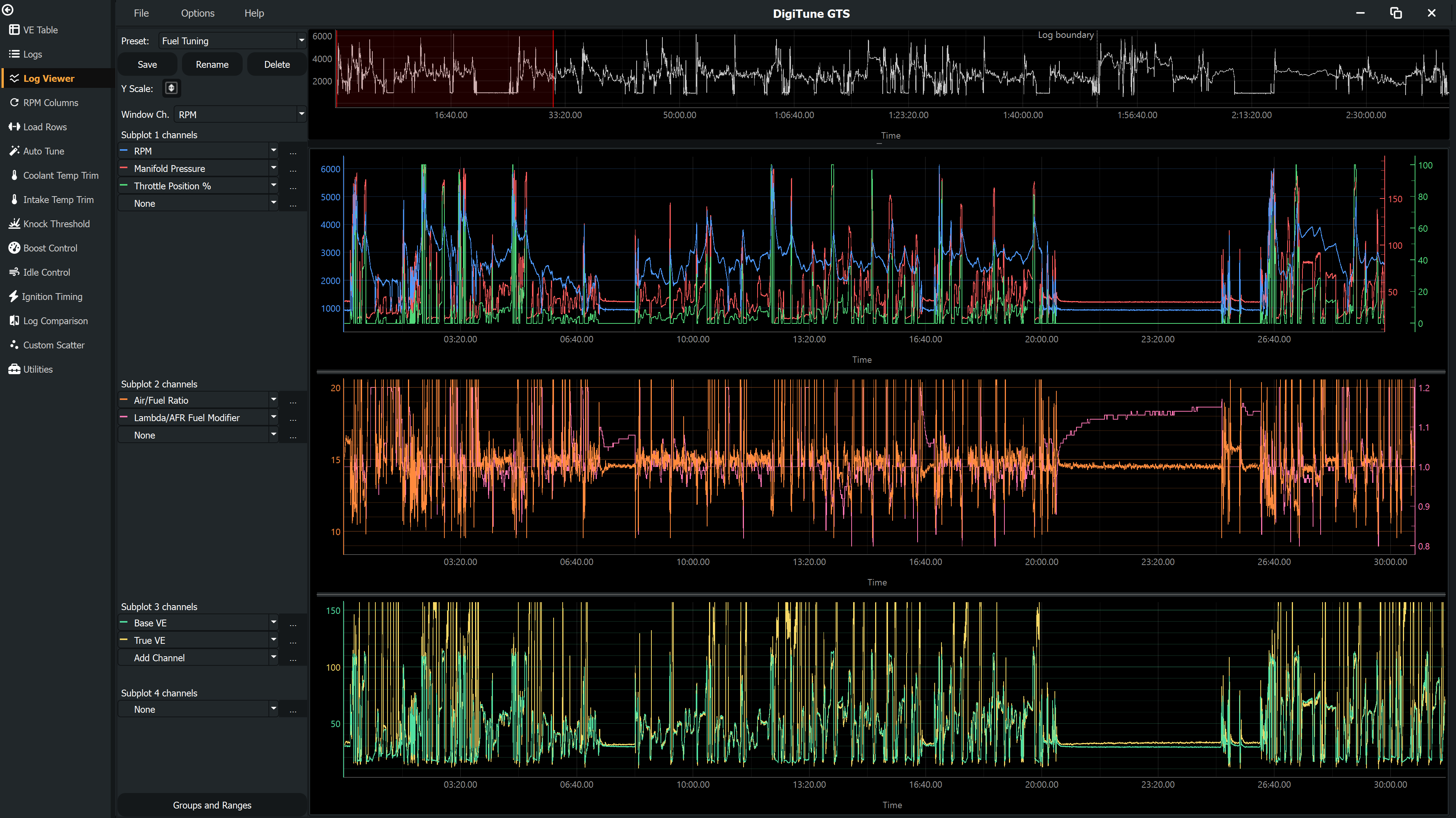
Overview plot

The narrow plot at the top of the page shows the entire log as a single curve. A highlighted region marks the section currently shown in the main graphs.

Drag the region to pan through the log without zooming.
Drag the edges of the region to zoom in or out.
Use the dropdown above the overview to choose which channel to display in this plot.

Main graphs

Up to three stacked subplots are shown below the overview, each capable of displaying up to five channels. All three subplots share the same time axis — panning or zooming one pan/zooms all of them simultaneously.

Each channel gets its own right-side Y axis with an independently scaled range. Channels can also be grouped so that a set of related channels (for example MAP and Target MAP, or AFR and Target AFR) share a single Y axis and stay visually comparable.

Resizing subplots

A thin drag handle appears between each pair of stacked subplots. Click and drag the handle up or down to redistribute vertical space between subplots without affecting the others.

Channel selection

The panel on the left lists the channel slots for each subplot (up to five channels per subplot, three subplots). For each slot, pick a channel from the dropdown. A None entry leaves the slot empty.

Available channels include:

Canonical (imported) channels — standard channels mapped from the log (RPM, MAP, TPS, CLT, IAT, AFR, Lambda, knock per cylinder, boost, idle duty, etc.). These are listed at the top of each dropdown.
Raw channels — any columns in the log that were not mapped to a canonical name. These are shown exactly as they appear in the log file and listed below the canonical channels.
Derived channels — computed from available channels: Load (kPa or %TPS), TrueVE, MAP error, and Idle error.

Per-channel options

A … button next to each selected channel opens a popup with that channel's appearance and axis settings:

Setting	Description
Colour	Override the auto-assigned trace colour.
Line width	Pen width for the channel's curve.
Marker	Point marker style (circle, square, triangle, diamond, plus, ×, or none).
Axis mode	Controls how the channel's Y axis is scaled: Window auto — fit to the visible time window (default for most channels). Window auto (clamped) — window-auto but capped by the channel's fixed range. Full auto — fit to the entire dataset, not just the visible window. Manual — your custom min/max, overridden by autoscale on each interaction. Fixed — your custom min/max, never autoscaled.

Channel options are saved as part of the active preset (see Presets).

Groups and fixed Y ranges

Click Groups & Ranges at the top of the channel panel to open a popup that controls two tool-wide settings:

Channel groups — Sets of channels that should share a single Y axis whenever they appear in the same subplot. Add channels to a group as chips; remove with the × on each chip. Useful for related signals (MAP / Target MAP, AFR / Target AFR, multiple knock cylinders).
Fixed Y-axis ranges — Channels that should always use a locked min/max rather than auto-scaling. Defaults are sensible (e.g. TPS 0–100, AFR 9–20, MAP 0–250 kPa, Lambda 0.6–1.4), and any channel can be added or edited here.

Both lists are global (apply to every subplot) and persist between sessions.

Cursor and region selection

Cursor

Left-click anywhere on a graph to place a vertical cursor line. Drag the cursor to move it. The cursor label in the top-right corner of each subplot shows the exact time and value of every plotted channel at the cursor position. For status / enum channels (for example ME's WarmupState), the label decodes the integer to its text name.

Region selection (stats)

Click and drag horizontally on a subplot to shade an X range instead of placing a cursor. A stats panel appears in the corner showing min, max, mean, and standard deviation for every plotted channel over the selected window. Click outside the region to dismiss it. Cursor and region are mutually exclusive — placing a cursor clears any active region and vice versa.

Markers

Markers are user-placed vertical annotations on the time axis with a short description and colour. Right-click on a subplot at the time of interest and choose Add Marker to create one; click an existing marker line to edit its description, change colour, or delete it.

Markers persist depending on the source log file:

HDF5 logs (.h5 / .hdf5) — markers are written into the file itself in a /markers group.
Other log formats — markers are in-memory only by default. Enable Create JSON Sidecar for Markers in Settings to write a <log>.markers.json file alongside the source log.
Multiple logs loaded together — markers stay in-memory only, since there is no single "owner" log for a marker at a merged X position.

Multiple logs and boundaries

When more than one log is loaded and included, DigiTune GTS merges them end-to-end into a single continuous timeline. Dashed vertical lines mark the point where each log ends and the next begins, so it is always clear which part of the combined view came from which session.

Time axis display

The time axis can be displayed in three ways, selectable from Settings → Log Viewer → Time Axis Display:

Elapsed seconds — seconds from the start of the log (or merged dataset).
HH:MM:SS since log start — hours/minutes/seconds since start (default).
Wall clock — absolute time of day, parsed from the log filename if present, else taken from the file's modification time.

Performance: downsampling

On dense logs (many hundreds of thousands of samples) plotting every sample can be slow. The Downsampling Mode setting controls how channels are reduced to screen pixels:

None (default) — render every sample. Slow on million-sample logs but lossless.
Min/max — preserve every spike; recommended for finding transients.
Mean — smooths noise but may flatten short transients.
Subsample — fastest, but can miss narrow spikes.

Additional viewer settings (gridlines, hidden intermediate time axes, marker sidecars) are in Settings → Log Viewer.

Presets

A preset saves your current channel selection, overview channel, and all per-channel options. It does not save the time window — only which channels are active and how they look.

Saving a preset

Configure the channels and options you want to display.
Click Save in the Preset row.
Enter a name for the preset and confirm. To overwrite an existing preset, choose the same name.

Loading a preset

Pick the preset from the Preset dropdown. The channel selection and options update immediately. If you edit channels after loading, a modified entry is added to the dropdown so you can switch back to the on-disk version without losing your in-progress changes.

Renaming and deleting

Rename renames the currently selected preset on disk. Delete removes it. Preset files are stored in %LOCALAPPDATA%\DigiTune\GTS\LogViewerPresets\; a small set of defaults is copied there on first run.

Auto-applied presets from warnings

When a log warning is raised (knock, lost sync, voltage instability, AFR sensor failure, etc.), clicking the warning's View link in the warnings dialog opens the Log Viewer with the most relevant preset pre-loaded (for example, Knock Analysis or AFR) so the suspect signals are on screen immediately. If a preset of that name does not exist, a sensible default is created.